contourslice

Draw contours in volume slice planes

Syntax

*

contourslice(X,Y,Z,V,Sx,Sy,Sz)
contourslice(X,Y,Z,V,Xi,Yi,Zi)
contourslice(V,Sx,Sy,Sz), contourslice(V,Xi,Yi,Zi)
contourslice(...,n)
contourslice(...,cvals)
contourslice(...,[cv cv])
contourslice(...,'method')
h = contourslice(...)

Description

contourslice(X,Y,Z,V,Sx,Sy,Sz) draws contours in the x-, y-, and z-axis aligned planes at the points in the vectors Sx, Sy, Sz. The arrays X, Y, and Z define the coordinates for the volume V and must be monotonic and 3-D plaid (such as the data produced by meshgrid). The color at each contour is determined by the volume V, which must be an m-by-n-by-p volume array.

contourslice(X,Y,Z,V,Xi,Yi,Zi) draws contours through the volume V along the surface defined by the arrays Xi,Yi,Zi.

contourslice(V,Sx,Sy,Sz) and contourslice(V,Xi,Yi,Zi) (omitting the X, Y, and Z arguments) assumes [X,Y,Z] = meshgrid(1:n,1:m,1:p) where [m,n,p]= size(v).

contourslice(...,n) draws n contour lines per plane, overriding the automatic value.

contourslice(...,cvals) draws length(cval) contour lines per plane at the values specified in vector cvals.

contourslice(...,[cv cv]) computes a single contour per plane at the level cv.

contourslice(...,'method') specifies the interpolation method to use. method can be: linear, cubic, nearest. nearest is the default except when the contours are being drawn along the surface defined by Xi, Yi, Zi, in which case linear is the default (see interp3 for a discussion of these interpolation methods).

h = contourslice(...) returns a vector of handles to patch objects that are used to implement the contour lines.

Examples

This example uses the flow data set to illustrate the use of contoured slice planes (type doc flow for more information on this data set). Notice that this example:

* Specifies a vector of length = 9 for Sx, an empty vector for the Sy, and a scalar value (0) for Sz. This creates nine contour plots along the x direction in the y-z plane, and one in the x-y plane at z = 0.
* Uses linspace to define a ten-element linearly spaced vector of values from -8 to 2 that specifies the number of contour lines to draw at each interval.
* Defines the view and projection type (camva, camproj, campos)
* Sets figure (gcf) and axes (gca) characteristics.
o

[x y z v] = flow;
h = contourslice(x,y,z,v,[1:9],[],[0],linspace(-8,2,10));
axis([0,10,-3,3,-3,3]); daspect([1,1,1])
camva(24); camproj perspective;
campos([-3,-15,5])
set(gcf,'Color',[.5,.5,.5],'Renderer','zbuffer')
set(gca,'Color','black','XColor','white', ...
'YColor','white','ZColor','white')
box on




contrast

Grayscale colormap for contrast enhancement

Syntax

*

cmap = contrast(X)
cmap = contrast(X,m)

Description

The contrast function enhances the contrast of an image. It creates a new gray colormap, cmap, that has an approximately equal intensity distribution. All three elements in each row are identical.

cmap = contrast(X) returns a gray colormap that is the same length as the current colormap.

cmap = contrast(X,m) returns an m-by-3 gray colormap.

Examples

Add contrast to the clown image defined by X.

*

load clown;
cmap = contrast(X);
image(X);
colormap(cmap);


conv

Convolution and polynomial multiplication

Syntax

*

w = conv(u,v)

Description

w = conv(u,v) convolves vectors u and v. Algebraically, convolution is the same operation as multiplying the polynomials whose coefficients are the elements of u and v.

Definition

Let m = length(u) and n = length(v). Then w is the vector of length m+n-1 whose kth element is




The sum is over all the values of j which lead to legal subscripts for u(j) and v(k+1-j), specifically j = max(1,k+1-n): min(k,m). When m = n, this gives

*

w(1) = u(1)*v(1)
w(2) = u(1)*v(2)+u(2)*v(1)
w(3) = u(1)*v(3)+u(2)*v(2)+u(3)*v(1)
...
w(n) = u(1)*v(n)+u(2)*v(n-1)+ ... +u(n)*v(1)
...
w(2*n-1) = u(n)*v(n)

Algorithm

The convolution theorem says, roughly, that convolving two sequences is the same as multiplying their Fourier transforms. In order to make this precise, it is necessary to pad the two vectors with zeros and ignore roundoff error. Thus, if

*

X = fft([x zeros(1,length(y)-1)])

and

*

Y = fft([y zeros(1,length(x)-1)])

then conv(x,y) = ifft(X.*Y)




conv2

Two-dimensional convolution

Syntax

*

C = conv2(A,B)
C = conv2(hcol,hrow,A)
C = conv2(...,'shape')

Description

C = conv2(A,B) computes the two-dimensional convolution of matrices A and B. If one of these matrices describes a two-dimensional finite impulse response (FIR) filter, the other matrix is filtered in two dimensions.

The size of C in each dimension is equal to the sum of the corresponding dimensions of the input matrices, minus one. That is, if the size of A is [ma,na] and the size of B is [mb,nb], then the size of C is [ma+mb-1,na+nb-1].

C = conv2(hcol,hrow,A) convolves A first with the vector hcol along the rows and then with the vector hrow along the columns. If hcol is a column vector and hrow is a row vector, this case is the same as C = conv2(hcol*hrow,A).

C = conv2(...,'shape') returns a subsection of the two-dimensional convolution, as specified by the shape parameter:

full
Returns the full two-dimensional convolution (default).
same
Returns the central part of the convolution of the same size as A.
valid
Returns only those parts of the convolution that are computed without the zero-padded edges. Using this option, C has size [ma-mb+1,na-nb+1] when all(size(A) >= size(B)). Otherwise conv2 returns [].

Algorithm

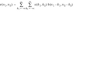
conv2 uses a straightforward formal implementation of the two-dimensional convolution equation in spatial form. If a and b are functions of two discrete variables,a and b, then the formula for the two-dimensional convolution of and is



In practice however, conv2 computes the convolution for finite intervals.

Note that matrix indices in MATLAB always start at 1 rather than 0. Therefore, matrix elements A(1,1), B(1,1), and C(1,1) correspond to mathematical quantities a(0,0), b(0,0), and c(0,0).